Basic User Guide
The SLSQP algorithm is designed to minimize a scalar objective function
of one or more variables, subject to constraints.
The optimize() function is a wrapper to the original SLSQP
implementation by Dieter Kraft [Kra88, Kra94].
The PySLSQP wrapper provides a slightly modified interface to the
optimization problem and many additional features, compared to the Scipy wrapper.
The optimize function solves the general nonlinear programming problem:
where \(x\) is the vector of optimization variables with size \(n\), \(f(x)\) is the scalar objective function, \(c(x)\) is the vector-valued constraint function, and \(xl\) and \(xu\) are vectors of lower and upper bounds, respectively. The first \(meq\) constraints are equalities while the remaining \( (m - meq) \) constraints are inequalities.
Defining your optimization problem
We previously looked at a very simple example in the Getting Started section.
Now, let’s look at a more complex problem that has both equality and inequality constraints, with variable bounds.
Here, we aim to minimize x^2 + y^2
subject to the constraints x+y=1 and 3x+2y>=1, with the bounds x>=0.4 and y<=0.6.
Now we write this example in the standard problem format shown above for SLSQP:
The code below defines the computation for the objective, constraint and their derivatives. It also defines the initial guess \(x0\) and other problem variables such as \(meq\), \(xl\), and \(xu\).
import numpy as np

# "x" represents the vector of optimization variables
def objective(x):
    # the objective function
    return x[0]**2 + x[1]**2

def gradient(x):
    # the gradient of the objective function
    return np.array([2*x[0], 2*x[1]])

def constraints(x):
    # the constraint functions formulated as c_eq(x) = 0, c_ineq(x) >= 0
    return  np.array([x[0] + x[1] - 1, 3*x[0] + 2*x[1] - 1])

def jacobian(x):
    # the jacobian of the constraint functions
    return np.array([[1, 1], [3, 2]])

# lower bounds on the optimization variables
x_lower = np.array([0.4, -np.inf])
# upper bounds on the optimization variables
x_upper = np.array([np.inf, 0.6])
# number of equality constraints (at the beginning of the constraint vector)
num_eqcon = 1

x0 = np.array([2,3])
Solving the optimization problem
We now import the optimize() function that actually runs the SLSQP algorithm and call it with the problem variables
and functions defined above.
If the derivatives grad and/or jac is not provided, optimize() will estimate them using finite differencing.
See Other optimizer options for specifying custom steps for finite difference approximation.
Once optimize is executed, the summary of the final optimization results will be printed on the console by default.
The function returns a dictionary that holds the results of the optimization.
A summary of the major iterations is also written to a file by default.
from pyslsqp import optimize

# optimize returns a dictionary that contains the results from optimization
results = optimize(x0, obj=objective, grad=gradient, con=constraints, jac=jacobian, meq=num_eqcon, xl=x_lower, xu=x_upper)
Optimization terminated successfully    (Exit mode 0)
            Final objective value                : 5.000000e-01
            Final optimality                     : 1.232595e-31
            Final feasibility                    : 0.000000e+00
            Number of major iterations           : 4
            Number of function evaluations       : 4
            Number of derivative evaluations     : 4
            Average Derivative evaluation time   : 0.000051 s per evaluation
            Average Function evaluation time     : 0.000036 s per evaluation
            Total Function evaluation time       : 0.000206 s [  5.43%]
            Total Derivative evaluation time     : 0.000142 s [  3.75%]
            Optimizer time                       : 0.000145 s [  3.82%]
            Processing time                      : 0.003300 s [ 86.99%]
            Visualization time                   : 0.000000 s [  0.00%]
            Total optimization time              : 0.003793 s [100.00%]
            Summary saved to                     : slsqp_summary.out
Viewing the results
We can print and see the returned results dictionary as shown below.
# print the returned "results" dictionary as a table
from pyslsqp.postprocessing import print_dict_as_table
print_dict_as_table(results)
--------------------------------------------------
        x                        : [0.5 0.5]
        objective                : 0.5
        optimality               : 1.232595164407831e-31
        feasibility              : 0.0
        constraints              : [0.  1.5]
        multipliers              : [1. 0.]
        gradient                 : [1. 1.]
        jacobian                 : [[1. 1.]
 [3. 2.]]
        num_majiter              : 4
        nfev                     : 4
        ngev                     : 4
        fev_time                 : 0.00020599365234375
        gev_time                 : 0.0001423358917236328
        optimizer_time           : 0.00014495849609375
        processing_time          : 0.003299713134765625
        visualization_time       : 0.0
        total_time               : 0.003793001174926758
        status                   : 0
        message                  : Optimization terminated successfully
        success                  : True
        summary_filename         : slsqp_summary.out
--------------------------------------------------
As seen from above, the summary of the optimization will be saved to slsqp_summary.out, unless the user provided
the summary_filename keyword argument for the optimize() function.
The contents of the summary file for the above optimization is shown below.
MAJOR  NFEV  NGEV           OBJFUN            GNORM            CNORM             FEAS              OPT             STEP
    0     1     1     4.360000E+00     4.176123E+00     6.403124E+00     9.900000E+01     9.900000E+01     9.900000E+01
    1     2     1     5.200000E-01     4.176123E+00     1.400000E+00     1.600000E+00     3.840000E+00     1.000000E+00
    2     3     2     5.022222E-01     1.442221E+00     1.533333E+00     4.440892E-16     7.697546E-16     1.000000E+00
    3     4     3     5.000000E-01     1.417353E+00     1.500000E+00     1.110223E-16     1.517305E-16     1.000000E+00
    4     4     4     5.000000E-01     1.414214E+00     1.500000E+00     0.000000E+00     1.232595E-31     1.000000E+00
The following table describes the different columns in the summary file.
Column # |
Header |
Description |
|---|---|---|
1 |
MAJOR |
Major iteration number |
2 |
NFEV |
Number of function (obj, con) evaluations |
3 |
NGEV |
Number of derivative (grad, jac) evaluations |
4 |
OBJFUN |
Objective function value |
5 |
GNORM |
Norm of the objective gradient |
6 |
CNORM |
Norm of the constraint vector |
7 |
FEAS |
Feasibility measure |
8 |
OPT |
Optimality measure |
9 |
STEP |
Step length taken after line search |
Scaling a problem
We can also scale the problem defined above without changing any of the previous definitions.
The optimize function can independently scale the optimization variables, objective and constraint functions using
user-provided arguments for x_scaler, obj_scaler, and con_scaler as shown below.
Here, we scale the optimization variables \(x_1\) and \(x_2\) by a factor of \(10\) and \(0.1\) respectively.
The objective function \(f\) is scaled by a factor of \(0.01\) whereas the constraint functions \(c_i\) are all
scaled by \(2000\).
For \(x\) and \(c\), we can scale all the entries differently by inputting a vector-valued scaler,
or scale them by the same value by inputting a scalar-valued scaler.
x_sc = np.array([10., 0.1])
f_sc = 0.01
c_sc = 2000
results = optimize(x0, obj=objective, grad=gradient, con=constraints, jac=jacobian,
                   meq=num_eqcon, xl=x_lower, xu=x_upper,
                   x_scaler=x_sc, obj_scaler=f_sc, con_scaler=c_sc,
                   summary_filename="scaled_summary.out")

print_dict_as_table(results)
Optimization terminated successfully    (Exit mode 0)
            Final objective value                : 5.000000e-01
            Final optimality                     : 7.682743e-16
            Final feasibility                    : 3.841372e-14
            Number of major iterations           : 9
            Number of function evaluations       : 10
            Number of derivative evaluations     : 9
            Average Derivative evaluation time   : 0.000066 s per evaluation
            Average Function evaluation time     : 0.000071 s per evaluation
            Total Function evaluation time       : 0.000662 s [  7.51%]
            Total Derivative evaluation time     : 0.000643 s [  7.29%]
            Optimizer time                       : 0.001009 s [ 11.45%]
            Processing time                      : 0.006499 s [ 73.75%]
            Visualization time                   : 0.000000 s [  0.00%]
            Total optimization time              : 0.008812 s [100.00%]
            Summary saved to                     : scaled_summary.out
--------------------------------------------------
        x                        : [0.5 0.5]
        objective                : 0.49999999999996164
        optimality               : 7.682743330406234e-16
        feasibility              : 3.8413716652030416e-14
        constraints              : [-3.84137167e-14  1.50000000e+00]
        multipliers              : [5.e-06 0.e+00]
        gradient                 : [1. 1.]
        jacobian                 : [[1. 1.]
 [3. 2.]]
        num_majiter              : 9
        nfev                     : 10
        ngev                     : 9
        fev_time                 : 0.0006620883941650391
        gev_time                 : 0.0006425380706787109
        optimizer_time           : 0.001008749008178711
        processing_time          : 0.006498813629150391
        visualization_time       : 0.0
        total_time               : 0.008812189102172852
        status                   : 0
        message                  : Optimization terminated successfully
        success                  : True
        summary_filename         : scaled_summary.out
--------------------------------------------------
Notice that it took more iterations than before for the algorithm to converge and the results are not exactly the same as in the case without scaling.
Note
The optimality, feasibility, and multipliers shown are for the scaled problem, whereas the optimization variables, objective, constraints, and gradients are for the unscaled problem.
We also set summary_filename=scaled_summary.out when calling optimize() this time and
the optimization summary is now saved in a different file which is shown below.
MAJOR  NFEV  NGEV           OBJFUN            GNORM            CNORM             FEAS              OPT             STEP
    0     1     1     4.360000E+00     4.176123E+00     6.403124E+00     9.900000E+01     9.900000E+01     9.900000E+01
    1     2     1     4.997361E+00     4.176123E+00     2.999560E+00     3.200000E+03     6.392961E-03     1.000000E+00
    2     4     2     4.993763E+00     4.019589E+00     2.998960E+00     1.598790E+03     1.595809E-02     1.000000E+00
    3     5     3     4.990164E+00     4.469346E+00     2.998360E+00     2.220446E-13     2.213144E-18     1.000000E+00
    4     6     4     4.972198E+00     4.467735E+00     2.995359E+00     6.661338E-13     6.624715E-18     1.000000E+00
    5     7     5     4.883084E+00     4.459685E+00     2.980386E+00     2.220446E-13     2.189196E-18     1.000000E+00
    6     8     6     4.455183E+00     4.419540E+00     2.906269E+00     1.332268E-12     1.258534E-17     1.000000E+00
    7     9     7     2.722830E+00     4.221461E+00     2.554237E+00     5.329071E-12     3.988090E-17     1.000000E+00
    8    10     8     5.000000E-01     3.300200E+00     1.500000E+00     2.575717E-11     1.607718E-16     1.000000E+00
    9    10     9     5.000000E-01     1.414214E+00     1.500000E+00     7.682743E-11     7.682743E-16     1.000000E+00
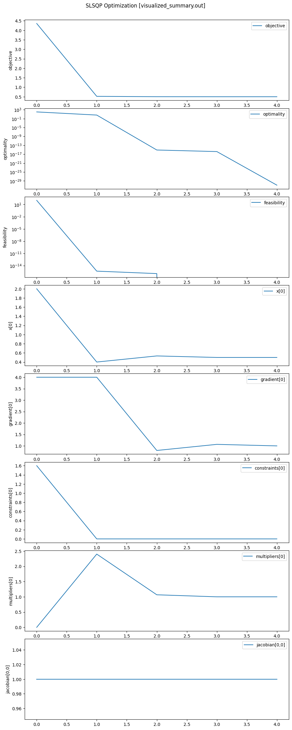
Live Visualization
To visualize the progression of values of scalar variables in real time during the optimization, set visualize=True.
By default, the list of variables to visualize is set as visualize_vars=['objective', 'optimality', 'feasibility'].
The complete list of variables that are available for visualization is
['x[i]', 'objective', 'optimality', 'feasibility', 'constraints[i]', 'gradient[i]', 'multipliers[i]', 'jacobian[i,j]'],
where i and j denote the indices of the the respective variable array and is necessary since only
scalar variables can be visualized.
To keep the plot window open after optimization, set keep_plot_open=True when calling optimize().
The name of the file where the final optimization plot is saved can be set using the keyword argument
save_figname which is set by default as save_figname="slsqp_plot.pdf".
The following example plots the objective \(f(x)\), optimality, feasibility, the optimization variable \(x_1\), the objective gradient \(\frac{\partial f}{\partial x_1}(x)\), the constraint \(c_1(x)\), the Lagrange multiplier corresponding to the constraint \(c_1(x)\), and the constraint derivative \(\frac{\partial c_1}{\partial x_1}(x)\).
%matplotlib inline

results = optimize(x0, obj=objective, grad=gradient, con=constraints, jac=jacobian,
                   meq=num_eqcon, xl=x_lower, xu=x_upper,
                   visualize=True, visualize_vars=['objective', 'optimality', 'feasibility', 'x[0]', 'gradient[0]', 'constraints[0]', 'multipliers[0]', 'jacobian[0,0]'],
                   summary_filename="visualized_summary.out", keep_plot_open=True)
Optimization terminated successfully    (Exit mode 0)
            Final objective value                : 5.000000e-01
            Final optimality                     : 1.232595e-31
            Final feasibility                    : 0.000000e+00
            Number of major iterations           : 4
            Number of function evaluations       : 4
            Number of derivative evaluations     : 4
            Average Derivative evaluation time   : 0.000033 s per evaluation
            Average Function evaluation time     : 0.000036 s per evaluation
            Total Function evaluation time       : 0.000132 s [  0.00%]
            Total Derivative evaluation time     : 0.000146 s [  0.01%]
            Optimizer time                       : 0.000093 s [  0.00%]
            Processing time                      : 0.002785 s [  0.10%]
            Visualization time                   : 2.808829 s [ 99.89%]
            Total optimization time              : 2.811984 s [100.00%]
            Summary saved to                     : visualized_summary.out
            Plot saved to                        : slsqp_plot.pdf
Unlike in the console outputs from previous examples, see that “Visualization time” is nonzero now. It is worth noting that visualization takes up most of time in smaller problems. For example, in the problem above, \(99.8 \%\) of the total optimization time is spent on visualization.
Writing optimization data to a file
To save the data and variables generated during the optimization iterations, set save_itr=all or save_itr=major when calling optimize().
This will save the variables in the list defined by save_vars after every iteration if save_itr=all, or after each major iteration if save_itr=major.
By default, save_vars=['x', 'objective', 'optimality', 'feasibility', 'step', 'iter', 'majiter', 'ismajor', 'mode'].
However, the user can specify any subset of variables from the list
['x', 'objective', 'optimality', 'feasibility', 'step', 'mode', 'iter', 'majiter', 'ismajor', 'constraints', 'gradient', 'multipliers', 'jacobian'].
The user can also specify the name of file where the data is saved using the save_filename keyword argument.
The default name for the save file is slsqp_recorder.hdf5, and the data is always stored in the hdf5 file format.
We now use the same example as before to save the optimization variables with their corresponding major iteration using save_itr='major' and save_var=['majiter', 'x'].
We will save the data to a file named save_file.hdf5.
results = optimize(x0, obj=objective, grad=gradient, con=constraints, jac=jacobian,
                   meq=num_eqcon, xl=x_lower, xu=x_upper,
                   save_itr='major', save_vars=['majiter', 'x'],
                   save_filename="save_file.hdf5")
Optimization terminated successfully    (Exit mode 0)
            Final objective value                : 5.000000e-01
            Final optimality                     : 1.232595e-31
            Final feasibility                    : 0.000000e+00
            Number of major iterations           : 4
            Number of function evaluations       : 4
            Number of derivative evaluations     : 4
            Average Derivative evaluation time   : 0.000048 s per evaluation
            Average Function evaluation time     : 0.000074 s per evaluation
            Total Function evaluation time       : 0.000193 s [  1.19%]
            Total Derivative evaluation time     : 0.000296 s [  1.83%]
            Optimizer time                       : 0.000125 s [  0.77%]
            Processing time                      : 0.015592 s [ 96.21%]
            Visualization time                   : 0.000000 s [  0.00%]
            Total optimization time              : 0.016206 s [100.00%]
            Summary saved to                     : slsqp_summary.out
            Iteration data saved to              : save_file.hdf5
The console output above now tells us that the iteration data is saved to “save_file.hdf5”. For more details on accessing the saved data or using the saved data for visualization or hot/warm start, see Post-processing.
Other optimizer options
The following table describes some of the other options that could be set while calling optimize.
Option |
Type (default value) |
Description |
|---|---|---|
|
int (100) |
Maximum number of iterations. |
|
float (1e-6) |
|acc| is the stopping criterion and controls the final accuracy. |
|
int (1) |
Controls the verbosity of the SLSQP algorithm. |
|
bool (False) |
If True, the plot window will remain open after optimization. |
|
str (“slsqp_plot.pdf”) |
The name of the file to which the final plot will be saved. |
|
np.ndarray or float (None) |
The absolute step size to use for numerical approximation of the derivatives. |
|
np.ndarray or float |
The relative step size to use for numerical approximation of the derivatives. |
|
callable (None) |
Function to be called after each major iteration. |
To get the complete list of options for optimize() and their default values as a dictionary, run get_default_options() as shown below.
from pyslsqp import get_default_options

options = get_default_options()
print_dict_as_table(options)
--------------------------------------------------
        obj                      : None
        grad                     : None
        con                      : None
        jac                      : None
        meq                      : 0
        callback                 : None
        xl                       : None
        xu                       : None
        x_scaler                 : 1.0
        obj_scaler               : 1.0
        con_scaler               : 1.0
        maxiter                  : 100
        acc                      : 1e-06
        iprint                   : 1
        finite_diff_abs_step     : None
        finite_diff_rel_step     : 1.4901161193847656e-08
        summary_filename         : slsqp_summary.out
        warm_start               : False
        hot_start                : False
        load_filename            : None
        save_itr                 : None
        save_filename            : slsqp_recorder.hdf5
        save_vars                : ['x', 'objective', 'optimality', 'feasibility', 'step', 'iter', 'majiter', 'ismajor', 'mode']
        visualize                : False
        visualize_vars           : ['objective', 'optimality', 'feasibility']
        keep_plot_open           : False
        save_figname             : slsqp_plot.pdf
--------------------------------------------------
For postprocessing saved data, see Post-processing.
For the complete API of PySLSQP, visit the API Reference.